WebAssembly Edge Model for learning English, built for low-end device

  • Ref: https://github.com/quochung-cyou/virulen

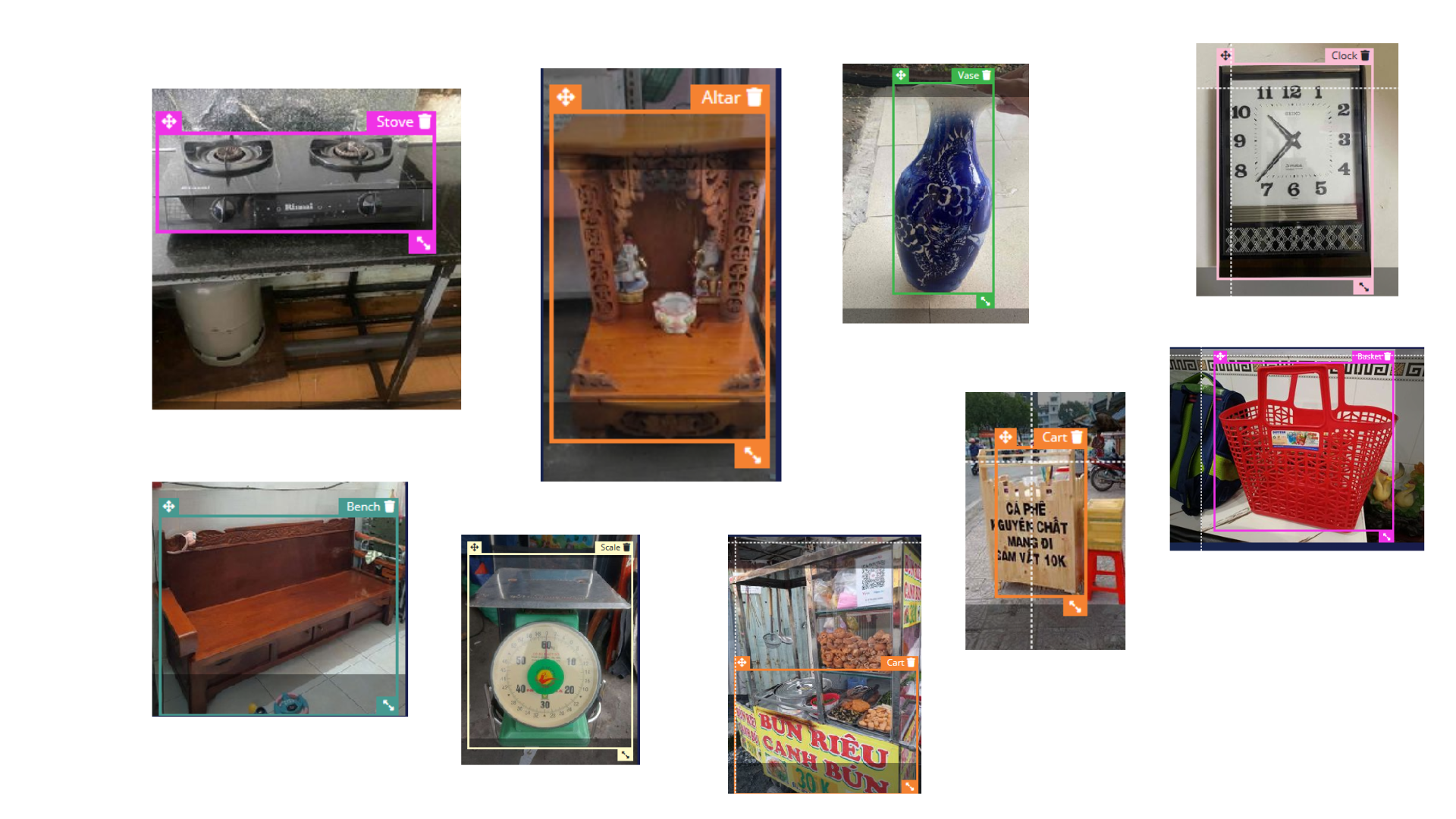
Virulen (VietLens) is a PWA English-learning app that lets learners in Vietnam point their camera at real-world objects and instantly see their English word, Vietnamese meaning, pronunciation, and example sentences.

Instead of memorizing words from Western textbooks, learners build a collection of cards from the everyday objects around them – plastic stools, rice cookers, street food, school furniture – the real Vietnam.

Novelty:

  • New dataset for Vietnam-specific objects (10k data) in unconstrained environment
  • The app running fully offline in mid-end devices via webapp (which allow both IOS/Android/and any devices with web browser) to run. Benchmark showcase it interface with 200-300ms latency.

Label Tool Build Around Edge Impulse: https://github.com/quochung-cyou/label-tool-edgeimpulse

1. Why This Exists

Tourism & communication

  • Vietnam welcomed 12.6M+ international visitors in 2023 (VNAT), but tourism is still concentrated in major cities.
  • Reports from World Bank, VNExpress, Tuoi Tre highlight that many rural destinations stay “off the map” because of communication and English barriers, not because they lack beauty or culture.

English education, but out-of-context

  • Vietnamese students start English in Grade 1 (MOET curriculum), yet textbooks and apps are dominated by urban/Western objects.
  • A 2022 analysis in Asia TEFL Journal found that over 80% of vocabulary objects in mainstream textbooks are generic or Western (e.g., sofa, burger, subway) rather than local Vietnamese items.
  • Research by Vietnamese educators shows textbook gaps for things tourists actually see:
    • cái chõ xôi (sticky rice steamer)
    • ghế nhựa (red plastic stool)
    • quán cóc (street stall)
    • mâm cơm (family meal tray)

The result is a visual and cultural mismatch: “Chair” in the book is a Western dining chair; “chair” in real life is a plastic stool or bamboo bench. Students memorize the word, but it doesn’t connect to their reality.

Gap in current apps

  • Language apps (Duolingo, Memrise, Babbel, Ling, etc.) teach generic vocab; no offline, Vietnam-specific scan-and-learn for local objects.
  • Global datasets and routines miss Vietnam‑specific foods, tools, and rural scenes.

Virulen / VietLens targets this exact gap: Offline-first, locally trained object recognition + English learning, optimized for low-end Android devices in Vietnam.

2. How It Works

alt text

The large diagram below is the end‑to‑end pipeline that produces the on‑device model used in Virulen.
To make it easier to understand, we break it into four stages.

3.1 Web crawl & candidate discovery

alt text

This block corresponds to the left side of the diagram.

  • Search engines (Bing / Google)
    We query public search APIs to discover pages and images that are likely to contain Vietnam‑specific objects (street food, local tools, rural scenes, etc.).
  • Crawl module
    • Core Logic orchestrates crawling and filtering.
    • Multiple Workers download pages and images in parallel.
    • Output is a large pool of candidate images plus metadata.

This stage answers: “What images from the web might show the Vietnam objects we care about?”


3.2 Data acquisition for Viet‑specific objects

alt text

This block is the middle bottom of the diagram.

  • The crawl output is filtered into Vietnam bias object data – images that show Vietnamese contexts and artifacts we want the model to recognize.
  • A data acquisition service:
    • Stores the raw images.
    • Groups them into samples (per object / per scene).
    • Prepares preview grids (as shown in the photo‑grid box in the diagram).

This stage answers: “Which of those images are actually useful for our Vietnam‑focused dataset?”


3.3 Labeling & human‑in‑the‑loop

alt text

This block is the bottom‑right.

  • Produce / Core Logic / Consumer
    • A small pipeline (shown with Kafka) feeds images into the labeling tools and collects labeled results.
    • Images flow through a Produce → Label → Consume cycle.
  • Labeling module (web UI)
    • Human labelers see each image (or grid of images).
    • They draw bounding boxes, assign class names, and validate / correct auto‑suggested labels.
  • Gemini fallback (bottom‑left box in the diagram)
    • A multimodal model (e.g. Gemini 2.0 Flash) can propose initial labels.
    • Humans confirm or fix them instead of labeling everything from scratch.

This stage answers: “How do we turn raw images into high‑quality labeled training data?”


3.4 Edge Impulse training & deployment

alt text

This block is the top pipeline and the central Edge Impulse logo.

  • Model pipeline in Edge Impulse Studio
    • Data ingestion: labeled samples are uploaded into Edge Impulse.
    • Feature generation: images are converted into feature vectors.
    • Model architecture & training:
      • A CNN / object‑detection network is configured (backbone, head, etc.).
      • Training, validation, and augmentation happen inside Edge Impulse Studio.
    • Quantization: the trained model is quantized for efficient on‑device inference (the “int8 model” box in the diagram).
  • Export to Virulen
    • Edge Impulse exports a standalone WebAssembly model bundle.
    • The bundle is placed under public/edge-impulse/ and loaded in the app by lib/edge-impulse-browser.ts.
    • ScanCamera uses this model to run real‑time detection directly in the browser.
  • Frontend framework: Next.js 16 App Router, React 19, TypeScript.
  • On-device AI:
    • lib/edge-impulse-browser.ts lazy-loads:
      • /edge-impulse/edge-impulse-standalone.js
      • /edge-impulse/run-impulse.js
    • ScanCamera (components/scan-camera.tsx):
      • Captures frames from getUserMedia video.
      • Packs pixels into feature vectors (lib/ei-image.ts).
      • Calls the Edge Impulse classifier and receives bounding-box detections.
      • Applies simple per-label non-max suppression to clean up overlapping boxes.
      • Maps detection labels to card definitions (lib/card-dictionary.ts → findCardByLabel).
  • State & storage:
    • User stats, streak, week progress, and collected cards are stored in localStorage (lib/storage.ts).
    • Cards are reconstructed from compact references + dictionary data to keep storage lightweight.
  • UI / UX:
    • Mobile-first layout (app/globals.css, shadcn-style components in components/ui).
    • Animated scan overlay and capture animation (components/detection-overlay.tsx, components/capture-card-animation.tsx).
    • Floating dock navigation (components/floating-dock.tsx).

3. What the App Does

Core experience

  • Scan objects with the camera
    • The app uses an Edge Impulse object-detection model loaded in the browser (lib/edge-impulse-browser.ts) to detect objects in real time.
    • Detections are mapped to curated word cards (lib/card-dictionary.json → lib/card-dictionary.ts).
  • Catch and collect vocabulary cards
    • Each recognized object becomes a Word Card (lib/card-types.ts, lib/word-data.ts):
      • English word
      • Vietnamese meaning
      • Phonetic / pronunciation
      • Example sentences
      • Category (e.g., household, food, school, transport)
      • User-captured images
  • Gamified dashboard (Home page)
    • Daily mission word / quest
    • Weekly progress heatmap (components/week-progress.tsx)
    • Streak, total time spent scanning, and recent scans (app/page.tsx, lib/storage.ts).
  • Card collection & details
    • Browse all collected cards (app/cards/page.tsx, components/beautiful-card-collection.tsx).
    • View detail for each word: meaning, examples, images, and favorites.
  • Offline-friendly PWA
    • Next.js PWA setup (app/manifest.ts, app/layout.tsx + SwRegister) with:
      • start_url: "/virulen/"
      • display: "standalone"
    • Edge Impulse model & runtime served from static assets under public/edge-impulse/.
    • Designed to run on low-spec phones with no stable internet.

4. Tech Stack

  • Framework: Next.js 16 (App Router, TypeScript)
  • Language: TypeScript, React 19
  • Styling: Tailwind CSS 4, custom mobile-focused CSS, shadcn/ui components, Lucide icons
  • AI / CV: Edge Impulse WebAssembly classifier, custom Vietnam-focused dataset (served from public/edge-impulse)
  • Speech (optional): vosk-browser (script loaded in app/layout.tsx for browser speech recognition)
  • Storage: localStorage for cards, favorites, and stats
  • Animations: framer-motion, CSS animations

5. Getting Started

Prerequisites

  • Node.js ≥ 18
  • Package manager: pnpm (recommended), or npm.
  • A modern browser with camera support (for development).

Installation

# in the repo root
pnpm install
# or
npm install

Run in development

pnpm dev
# or
npm run dev

By default this runs on http://localhost:3000. Open it on a device with a camera (you can also use your laptop camera).

Note: In dev, base paths may differ from production (next.config.mjs uses basePath: "/virulen" and assetPrefix: "/virulen/" for static export).

Build & static export

This project is configured for static export:

pnpm build
# then
pnpm start   # Next.js standalone server

Or, if you run next export in your deployment pipeline, ensure you respect:

  • basePath: "/virulen"
  • assetPrefix: "/virulen/"
  • Static assets required for Edge Impulse under public/edge-impulse/.

6. Key Directories

  • app/
    • page.tsx – Home dashboard (stats, daily mission, quick actions, recent scans).
    • scan/page.tsx – Scan screen (integrates ScanCamera, current detections, “catch” animation).
    • cards/ – Card list and detail pages.
    • manifest.ts – PWA manifest.
    • layout.tsx – Root layout, fonts, PWA & speech scripts.
  • components/
    • scan-camera.tsx – Core camera + Edge Impulse pipeline.
    • detection-overlay.tsx – Renders bounding boxes.
    • beautiful-card-collection.tsx, word-card-item.tsx, word-card-modal.tsx – Collection UI.
    • floating-dock.tsx, stats-card.tsx, week-progress.tsx – Navigation and dashboard UI.
    • audio-recorder.tsx – Voice features (for pronunciation practice and missions).
  • lib/
    • edge-impulse-browser.ts – Loads and instantiates the Edge Impulse classifier.
    • ei-image.ts – Packs camera frames into features for the model.
    • card-dictionary.json – Dictionary of all supported words and metadata.
    • card-dictionary.ts / card-types.ts – Card models and helper functions.
    • storage.ts – Local storage for cards, favorites, and user stats.
    • asset-path.ts – Base path helper for static assets.
  • public/edge-impulse/
    • Edge Impulse generated files (edge-impulse-standalone.js, run-impulse.js, model assets).

7. Roadmap / Ideas

  • Richer Vietnam-specific dataset
    • Expand card-dictionary.json with more rural artifacts, foods, and tools.
    • Community-sourced images and labels from classrooms and local guides.
  • Education edition
    • Teacher dashboard: see which words a class has “caught”.
    • Thematic missions: “Market day”, “School day”, “Kitchen tour”.
  • Tourism bridge
    • Tourist mode: phrasebook + object scan for travelers.
    • Local mode: help locals explain cultural items to visitors (e.g., điếu cày, nón lá, bánh xèo).
  • Richer speech & pronunciation
    • Integrate vosk-browser fully for offline pronunciation practice and voice-based quizzes.
  • Data & research
    • Partner with educators and tourism experts to validate vocabulary lists.
    • Open data contributions (anonymized) to support further research on low-resource, domain-specific object recognition.
GOOSE 2D Fine-Grained Semantic Segmentation / ICRA 2026

  • Ref: https://github.com/quochung-cyou/goose-seg-icra2026

Approach to 64-class semantic segmentation on the GOOSE dataset. Final test score: 63.8 % composite mIoU on the ICRA 2026 Field Robotics Workshop Challenge.


Overview

The GOOSE (German Outdoor and Offroad Dataset) and its extension GOOSE-Ex contain images from three robotic platforms in unstructured outdoor environments. The task is pixel-level classification into 64 classes. Some classes are common (car, road, sky). Others are narrow (tree_root, barrel, kick_scooter). A few barely exist in the data.

Two model architectures, three augmentation strategies, test-time augmentation, and a greedy rule-learning ensemble are included. The repo contains training scripts, logs, and visualizations.


The data

GOOSE dataset splits below:

SplitImagesLabelsCamera
goose_2d_train~24,000yeswindshield_vis
goose_2d_val~556yeswindshield_vis
gooseEx_2d_train~4,500yescamera_left
gooseEx_2d_val~192yescamera_left
Test set~361noboth

Labels are grayscale PNGs where pixel value = class ID (0..63). Class 0 is undefined and counts toward metrics. No ignore index.

Class imbalance

Class imbalance is the top challenge. forest alone covers 20.7 % of all pixels. sky, asphalt, and low_grass together add another 36 %. Meanwhile pipe has roughly 1,852 pixels across the entire training set. barrel has 1,199. Several classes are so rare that models never learn them.

Class distribution

Rare class anatomy

Patches for the worst-performing classes (kick_scooter, barrier_tape, pipe, tree_root, motorcycle) are shown below. Most are tiny, occluded, or poorly lit.

Rare class grid

Methods

Models

Model 1: UPerHead with FlashInternImage-L (DCNv4 backbone)

FlashInternImage-L uses deformable convolutions v4. The UPerHead decoder fuses pyramid pooling with FPN-style features. An auxiliary FCN head on stage 3 provides extra gradient flow.

  • Backbone channels: 160, depths [5, 5, 22, 5]
  • Pretrained on ImageNet-22K → 1K at 384×384
  • Crop size: 2048×1024
  • Batch size: 2
  • 200,000 iterations, AdamW at 8e-4 with layer decay 0.94

Model 2: Mask2Former with the same backbone

Mask2Former uses a transformer decoder with 200 queries and a pixel decoder based on multi-scale deformable attention. Initialized from ADE20K weights (mask2former_flash_internimage_l_640_160k_ade20k_ss.pth) with manual handling of the 150 → 64 class mismatch. Training was slower per iteration (~2.1s vs ~0.9s) and stopped at ~47,000 iterations. Learning rate: 5e-5.

Augmentations

Standard MMSeg pipeline: random resize between 0.5x and 2.0x, random crop to 2048×1024, horizontal flip, photometric distortion, ImageNet normalization.

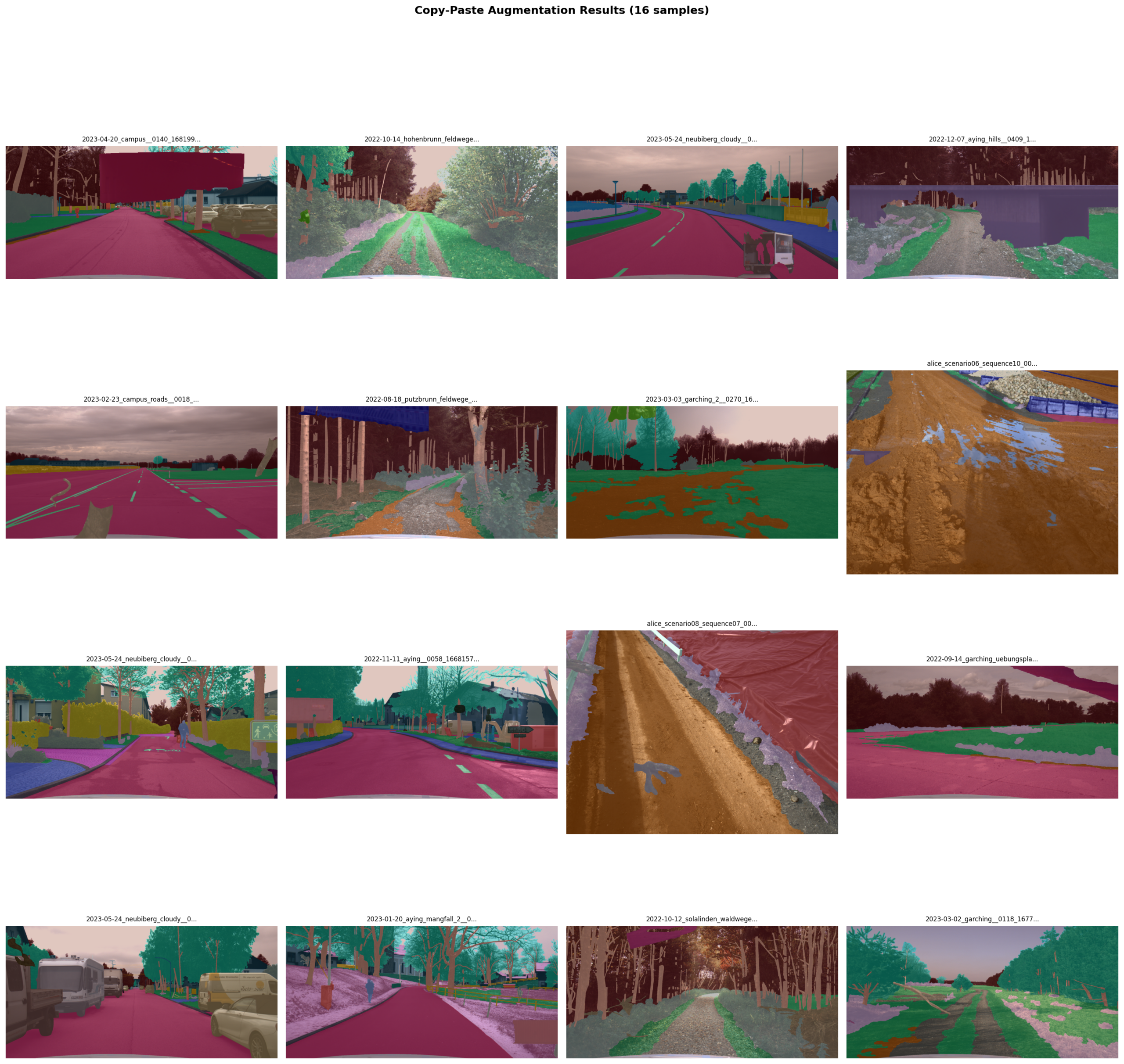
Copy-Paste: Instances of 17 rare classes extracted and pasted onto random target images with scaling from 0.2x to 4x. Two target images per source instance.

Copy-paste preview

Class weighting: Both models used ENet-style weights: 1 / log(1.02 + frequency), normalized and scaled to 64.

Test-time augmentation

Multi-scale inference at [0.75, 1.0, 1.25, 1.5] with horizontal flipping.

Ensemble

Model 1 (UPerHead) outperformed Model 2 on validation: 51.71 % vs 46.85 % mIoU. M2 still won specific classes. street_light, for instance: M1 got 13.1 % IoU while M2 got 46.8 %.

Tuned rule ensemble: A 3D histogram H[m1_pred, m2_pred, ground_truth] built over the full validation set. For every pixel group where M1 predicts class i and M2 predicts class c, the question is whether overriding M1 with M2 improves mIoU. An atom is accepted only if:

  • At least 500 pixels were in the group
  • M2 was significantly more correct than M1 (precision margin 0.05)
  • No single class dropped more than 0.005 IoU
  • The gain exceeded 5e-5 on the validation set

The greedy search accepted 18 atoms across 10 rules. Examples:

  • If M2 says building and M1 says obstacle or pole, trust M2
  • If M2 says curb and M1 says fence, gravel, or low_grass, trust M2
  • If M2 says street_light and M1 says forest or pole, trust M2

M1 alone: 44.21 % mIoU on the tuning split. Tuned ensemble: 47.94 %. A +3.72 % gain from 18 pixel-level rules.


Training

Training ran on a single A100. M1 peaked around 58 GB memory. M2 was lighter at ~48 GB but slower.

Training curves

M1 converged to higher mIoU and stayed there. M2’s loss looked reasonable but validation metrics plateaued lower. Mask2Former likely needs more data, longer training, or a better initialization than the ADE20K transfer. The transformer decoder also consumes many iterations.


Results

Validation metrics

ApproachaAccmIoUmAcc
UPerHead (M1)87.19 %51.71 %61.41 %
Mask2Former (M2)84.52 %46.85 %60.23 %
Tuned ensemble87.19 %51.79 %61.41 %
Model comparison

The tuned ensemble edges out M1 by 0.08 % on validation. The real win is per-class. Some classes improved significantly.

Per-class IoU on validation

Top 30 classes by M1 IoU below. M1 dominates frequent classes like sky, asphalt, and forest. M2 is competitive on street_light, rider, and bicycle.

Per-class IoU

The scatter plot below shows log frequency against IoU for both models. Rare classes cluster near zero. sky sits alone at the top right. barrel is an outlier with high IoU despite low frequency because it has a consistent visual signature (yellow cylinders).

Frequency vs IoU

Radar chart

16 diverse classes spanning the frequency spectrum. M1 covers more area overall, but M2 bulges on street_light and bicycle.

Radar chart

Precision vs recall

Most points sit below the diagonal, meaning recall is the bottleneck. The model finds the class when it is present, but misses many pixels. sky and barrel are the exceptions — high precision, high recall, easy classes.

Precision vs recall

Error analysis

Confusion matrices

Row-normalized confusion for the top 20 frequent classes. Dark diagonals = good recall. Off-diagonal heat shows misclassification patterns.

M1: 

M2: 

Common misclassifications: tree_crown → forest, high_grass → low_grass, wall → building. The model struggles with fine-grained vegetation boundaries and architectural edges.

Model disagreement

M1 and M2 agree on 86.77 % of pixels. When they disagree, M1 wins 96 % of the time. The 4 % where M2 wins is where the ensemble gains come from.

Disagreement stacked

Highest disagreement rates are on wall, rock, rider, and moss. These are ambiguous classes with fuzzy boundaries.

Disagreement rate

Ensemble gains

The waterfall chart below shows each accepted atom’s contribution to mIoU. Most atoms give small gains. A few give large gains — notably the debris → soil rule and the fence → curb rule.

Ensemble waterfall

Per-class IoU changes from the tuned rules. Biggest winners: curb (+55.3 %), debris (+23.5 %), street_light (+20.2 %). Some classes drop slightly, but the guard rails prevent any single class from dropping severely.

Tuned gains

Qualitative results

Validation samples

Image, ground truth, M1, M2. M2 is visibly noisier on vegetation and road boundaries.

Validation sample 1
Validation sample 2
Validation sample 3
Validation sample 4
Validation sample 5

Test samples

No ground truth for the test set: image → M1 → M2 → tuned ensemble. The tuned rules shift predictions: building edges get cleaner, curb appears where M1 predicted fence, street_light appears where M1 predicted pole.

Test sample 1
Test sample 2
Test sample 3
Test sample 4
Test sample 5

Official test results

The numbers above are from local validation. The official challenge test set evaluation is below. Composite mIoU: 63.80 %.
Per-class mIoU on test set

IDClassmIoU (%)
0undefined25.56
1traffic_cone0.00
2snow67.67
3cobble87.26
4obstacle53.99
5leaves19.74
6street_light49.20
7bikeway0.00
8ego_vehicle91.97
9pedestrian_crossing0.00
10road_block71.51
11road_marking72.07
12car93.73
13bicycle70.06
14person86.77
15bus87.79
16forest70.40
17bush38.97
18moss1.27
19traffic_light70.61
20motorcycle42.61
21sidewalk66.88
22curb63.23
23asphalt92.28
24gravel31.68
25boom_barrier35.35
26rail_track78.25
27tree_crown53.52
28tree_trunk65.07
29debris25.62
30crops77.21
31soil61.59
32rider44.85
33animal30.41
34truck51.78
35on_rails84.62
36caravan80.90
37trailer27.69
38building85.81
39wall54.83
40rock20.05
41fence84.46
42guard_rail62.40
43bridge7.62
44tunnel0.00
45pole50.44
46traffic_sign70.61
47misc_sign70.84
48barrier_tape27.02
49kick_scooter1.44
50low_grass73.01
51high_grass59.68
52scenery_vegetation33.35
53sky97.54
54water51.23
55wire31.55
56outlier0.00
57heavy_machinery48.78
58container59.42
59hedge48.98
60barrel92.30
61pipe0.00
62tree_root0.00
63military_vehicle0.00

Per-category mIoU

CategorymIoU (%)
Animal30.41
Construction78.37
Human86.67
Object40.42
Road69.99
Sign72.07
Sky97.54
Terrain89.14
Vegetation93.39
Vehicle86.77
Water51.23

Overall

  • mIoU fine: 55.24 %
  • mIoU fine (coarse): 72.36 %
  • mIoU composite: 63.80 %

The test gap between validation and test is notable. Some classes improved (cobble, road_block, trailer), others collapsed (leaves, moss, rock). The test set likely has different scene distributions or lighting conditions. The 0 % classes remained 0 %. traffic_cone and pipe probably need external data or synthetic injection to improve.


Repo structure

FileWhat it does
train_segment_py.pyTrain UPerHead model. Full MMSeg config in Python.
train_mask2former_l.pyTrain Mask2Former. Handles ADE20K pretrained weights with class mismatch.
generate_submission.pyInference + submission packaging for UPerHead.
generate_submission_mask2former.pyInference + submission packaging for Mask2Former.
ensemble_submission_tuned.pyApply tuned_rules.py to test predictions.
tune_ensemble_v2.pyGreedy rule optimizer. Builds 3D histogram, selects atoms.
copypaste_augmentation.pyCopy-Paste augmentation for rare classes.
copypaste_config.pyConfig for Copy-Paste.

Setup & Installation

Steps to go from a fresh machine to running training or inference.

1. Hardware

ComponentMinimumRecommended
GPUNVIDIA A100 80 GBA100 80 GB or H100
GPU memory (train)~58 GB (UPerHead), ~48 GB (Mask2Former)80 GB
Host RAM64 GB128 GB
Disk space400 GB free500 GB+
CUDA capability>= 8.0 (Ampere)>= 8.0

Training ran on a single A100. The scripts are single-GPU. For inference only, a smaller GPU may work with reduced batch size or TTA disabled.

2. System dependencies

  • CUDA >= 11.7 with matching NVCC and cuDNN
  • GCC compatible with your CUDA (e.g. GCC 10–11 for CUDA 11.7)
  • Standard build tools: build-essential, git, wget

Check CUDA and NVCC:

nvidia-smi
nvcc --version

3. Python environment

Create the conda environment:

conda create -n dcnv4 python=3.10 -y
conda activate dcnv4

Install core deep-learning stack:

conda install pytorch torchvision pytorch-cuda=11.7 -c pytorch -c nvidia -y

Install OpenMMLab dependencies:

pip install -U openmim
mim install mmcv-full==1.5.0
mim install mmsegmentation==0.27.0
pip install timm==0.6.11 mmdet==2.28.1

Install remaining Python packages used by the scripts:

pip install opencv-python Pillow tqdm matplotlib scipy numpy pandas

4. Build the DCNv4 CUDA extension

The DCNv4 backbone requires a custom CUDA operator. It must be compiled from source: (The DCNv4 version in this repo is modified for compatibility with the current environment – A100 and newer cuda/python versions)

cd DCNv4/DCNv4_op
pip install -e .

If this fails, typical causes are:

  • CUDA_HOME not set: export CUDA_HOME=/usr/local/cuda
  • NVCC / GCC version mismatch
  • PyTorch CUDA version does not match system CUDA

Verify the build:

python -c "import DCNv4.ext; print('OK')"

5. Prepare the data

The GOOSE and GOOSE-Ex datasets are downloaded automatically by the preparation script. They need ~192 GB of disk space.

python prepare_combined_dataset.py

This creates the expected data/ tree:

data/
  goose_2d_train/
  goose_2d_val/
  gooseEx_2d_train/
  gooseEx_2d_val/
  goose_2d_train_copypaste/   # created by copypaste_augmentation.py
  goose_label_mapping.csv

7. Optional: pretrained weights

Pretrained backbones are downloaded automatically on first run from HuggingFace:

  • UPerHead backbone: flash_intern_image_l_22kto1k_384.pth
  • Mask2Former pretrained: mask2former_flash_internimage_l_640_160k_ade20k_ss.pth

To skip training and run inference only, download the best fine-tuned checkpoints and place them under checkpoints/goose_seg_dcnv4/ and checkpoints/goose_mask2former_l/.


Running things

The conda environment is dcnv4. Python 3.10, PyTorch, MMCV, MMSegmentation.

Train UPerHead:

conda run -n dcnv4 python train_segment_py.py > training.log 2>&1 &

Train Mask2Former:

conda run -n dcnv4 python train_mask2former_l.py > training_maskformer.log 2>&1 &

Generate validation predictions and submission:

conda run -n dcnv4 python generate_submission.py
conda run -n dcnv4 python generate_submission_mask2former.py

Tune the ensemble:

conda run -n dcnv4 python tune_ensemble_v2.py
conda run -n dcnv4 python ensemble_submission_tuned.py

Regenerate all README visuals:

conda run -n dcnv4 python generate_readme_visuals.py
conda run -n dcnv4 python generate_confusion_heatmap.py
conda run -n dcnv4 python generate_disagreement_chart.py
conda run -n dcnv4 python generate_pr_scatter.py
conda run -n dcnv4 python generate_test_side_by_sides.py

What worked and what didn’t

Worked:

  • UPerHead decoder. Simple, reliable, better mIoU than Mask2Former for this data.
  • Test-time augmentation. Reliable gains at no training cost.
  • Class weighting. Stabilized training on the long tail.
  • The tuned rule ensemble. +3.72 % mIoU from 18 atoms.

Didn’t work:

  • Mask2Former underperformed given its compute cost. Likely needs longer training or better hyperparameter tuning. The ADE20K initialization may not transfer well to outdoor offroad scenes.
  • Copy-Paste and oversampling helped a little, but could not fix the core issue: some classes have so few pixels that duplication does not create real signal.
  • 64 classes is too many for the data volume. Several classes (traffic_cone, pipe, tree_root, military_vehicle, kick_scooter) scored exactly 0.0 on test.

Not tried:

  • Hard example mining / OHEM
  • Boundary loss
  • Pseudo-labeling on the test set
  • Model distillation
  • 3D point cloud fusion (the dataset has LiDAR)
  • External datasets

Attempt to finetune SLM for solving RCA in 5G network data

Part I: Introduction & The RCA Problem Space

Modern mobile networks are complex systems requiring high reliability. However, despite monitoring, faults like hardware failures or software misconfigurations occur. While detecting a fault is straightforward, the main challenge is Root Cause Analysis (RCA) — finding the root cause of the symptoms to help engineers fix them.

This project replicates the paper (Reasoning Language Models for Root Cause Analysis in 5G Wireless Networks) https://arxiv.org/pdf/2507.21974

The Complexity of 5G O&M

Traditionally, RCA relied on expert-defined logical frameworks or “fault trees”. However, these methods don’t scale well with 5G network complexity. While standard machine learning (Decision Trees, SVMs, Neural Networks) has been used, these models often lack the interpretability and reasoning needed for critical infrastructure.

Defining the Objective: RCA as Probabilistic Inference

We treat RCA as a probabilistic inference task. Formally, the goal is to identify the most probable cause from a set of potential root causes , given:

  • ****: Network engineering parameters.
  • ****: User plane observations.
  • ****: Observed symptoms.

The objective is to solve for:

c^=arg⁡maxc∈Cp(c|U,Yt,st)

This mathematical formulation provides a framework, but modeling these intricate dependencies in real-world data is notoriously difficult. This implementation explores how domain-adapted, reasoning-enhanced Large Language Models (LLMs) can bridge this gap by providing structured, multi-step diagnostic explanations.

The TeleLogs Framework

To benchmark these capabilities, we utilize TeleLogs, a curated dataset of network troubleshooting scenarios with expert-level annotations. TeleLogs simulates a realistic 5G environment where a User Equipment (UE) moves through a region covered by multiple Base Stations (BSs), providing full visibility into network configurations and performance drops.


Part II: Dataset Architecture & Diagnostic Parameters

To perform effective RCA, the model must synthesize three distinct data streams: configuration parameters, time-series observations, and defined symptoms.

Symptom Definition: The 600 Mbps Threshold

In this study, diagnostic scenarios are centered around a specific symptom (st): a significant degradation in downlink throughput where the performance falls below 600 Mbps. This drop serves as the trigger for the analysis, requiring the model to identify if the cause is environmental, a misconfiguration, or a mobility issue.

Network Engineering Parameters (U)

The dataset provides a comprehensive view of the network topology through static configuration parameters. Key parameters used in our analysis include:

ParameterDescription
gNodeB ID / Cell IDUnique identifiers for the base station and cell.
Mechanical/Digital TiltThe vertical angle of the antenna, essential for coverage analysis.
Mechanical/Digital AzimuthThe horizontal direction of the antenna.
Beam ScenarioSpecific beamforming configurations that determine vertical beamwidth.
Height & PCIPhysical height of the antenna and the Physical Cell ID.
Beam ScenarioSpecific beamforming configurations that determine vertical beamwidth.

User Plane Drive Test Data (Yt)

This represents the dynamic interaction between the user and the network. The model analyzes the following time-series indicators:

  • Throughput (DL): The primary indicator of service quality.
  • RSRP & SINR: Measure the signal strength and quality of the serving cell.
  • Neighboring RSRP: Signal strength from the top-k neighbor cells, used to detect interference or handover opportunities.
  • Resource Blocks (PRBs): The amount of radio resources allocated to the user.

The Ground Truth: Root Cause Classes (C1–C8)

The implementation evaluates the model’s ability to classify symptoms into one of eight distinct categories:

  • C1: Excessive downtilt causing weak coverage.
  • C2: Over-shooting coverage (distance > 1 km).
  • C3: Better performance available on a neighboring cell.
  • C4: Interference from non-colocated co-frequency cells.
  • C5: PCI Mod 30 conflict causing reference signal overlap.
  • C6: Performance degradation due to frequent handovers.
  • C7: Misconfigured handover thresholds.
  • C8: Insufficient PRB allocation.

Part III: Baseline Evaluation

Before fine-tuning, I established a performance baseline using Qwen2.5-1.5B-Instruct.

The Benchmarking Protocol

I ran a zero-shot inference on the TeleLogs Phase 1 test dataset, which contains 864 scenarios. The model was prompted using the standard template to analyze user-plane data and site engineering parameters, then choose the most likely root cause from the eight predefined classes.

Initial Findings

The baseline results showed the model was mostly guessing based on simple patterns:

  • Total Accuracy: 10.53% (91/864 correct).
  • The C1 Bias: The model correctly identified C1 (Excessive Downtilt) 42.59% of the time but used it as a “catch-all” for errors. In the top 10 most frequent errors, the model predicted C1 for other classes (C6, C8, C7, C2, C3, C4, and C5) a total of 312 times.
  • Instruction Following: While the model often produced the correct format (the boxed answer), it lacked the underlying logic to connect the RSRP/SINR drops to specific mobility or interference issues.
  • Placeholders: For many classes (C2, C4, C5, C8), the accuracy hovered near 3%, indicating that the base model could not differentiate between various types of signal degradation.
analysis report baseline - quochung.cyou PTIT
- quochung.cyou PTIT

Part IV: Synthetic Data Generation Phase 1 — Reasoning Traces

To improve reasoning, I started the first phase of synthetic data generation. The goal was to create a dataset that demonstrates the Chain-of-Thought (CoT) required for RCA.

The Teacher Model: Qwen3-32B

I utilized Qwen3-32B as the high-reasoning agent. Its significantly larger parameter count and inherent reasoning capabilities allowed it to act as the “expert engineer”. Unlike the 1.5B model, the 32B model can synthesize the relationship between (Engineering Parameters) and (User Observations) more effectively.

CoT Prompting Strategy

I implemented a customized prompting strategy designed to guide the model through a structured diagnostic trajectory. The prompt forced the model to:

  1. Analyze Data: Explicitly list the throughput drops and serving cell changes.
  2. Eliminate Unlikely Causes: Systematically rule out causes—for example, ruling out C2 (distance) if the serving cell is far away.
  3. Validate via Reflection: Check for specific conflicts, such as the PCI Mod 30 check for interference.

Data Acquisition

Through this multi-agent pipeline, I harvested an initial set of 138 samples. Each sample consisted of the original network log paired with a detailed reasoning trace leading to the correct ground-truth answer. This dataset was intended to teach the 1.5B model how to think, rather than just what to predict.


Part V: Experiment 1 The First LoRA Attempt

With 138 high-quality reasoning traces, I initiated the first fine-tuning stage. The goal was to align the Qwen2.5-1.5B-Instruct model with the structured diagnostic patterns found in the synthetic dataset. Following the general recommendations for domain adaptation in the provided LoRA research , I established a baseline configuration to mirror the paper’s parameters where possible.

Configuration and Training Setup

  • LoRA Hyperparameters: r = 32, alpha = 32, dropout = 0.1
  • Learning Rate: 1e-6
  • Epochs: 10.
  • Targeting: Applied LoRA across all linear layers (Query, Key, Value, Projection, and MLP) to maximize the model’s capacity to absorb the new domain knowledge.

The Regression Reality: 8.91% Accuracy

The results were a stark contrast to expectations. Instead of improving upon the baseline, the model’s performance dropped to 8.91% (77/864 correct).

  • Placeholder Issues: A significant issue was the increase in “placeholder” predictions. In the top 10 error categories, 7 were instances where the model outputted a placeholder rather than a valid root cause.
  • Reduced Instruction Following: The model lost some ability to follow basic formatting instructions. Focusing on the reasoning traces caused the model to struggle with the required \boxed{} format.
  • Word Count Increase: The mean word count increased from 245 to 651 words, often containing circular logic without a valid conclusion.

Hypothesis: Sample Sparsity and Overfitting

My hypothesis for this failure was sample sparsity. 138 samples are likely insufficient for a 1.5B model to learn both the complex 5G domain rules and the specific “Elimination-based” or “Contradiction-based” prompting strategies used in the dataset. The model likely overfitted to the specific noise of those 138 examples rather than learning the underlying causal relationships.

analysis report 77 - quochung.cyou PTIT
- quochung.cyou PTIT

Part VI: Experiment 2 Scaling Sample Size

To address the sparsity issue identified in Experiment 1, I moved to scale the training data. If 138 samples caused overfitting, perhaps a larger, more diverse dataset would force the model to generalize the reasoning steps.

The 300-Sample Expansion

I re-ran the synthetic generation pipeline with the Qwen3-32B teacher model to reach 300 samples. I also ensured a more balanced distribution across the 8 root cause classes to prevent the model from defaulting to “C1” as it did in the baseline.

Results: Marginal Recovery (9.61%)

Training the 1.5B model on 300 samples yielded a slight recovery but remained below the zero-shot baseline:

  • Total Accuracy: 9.61% (83/864).
  • Improved Class Recognition: Accuracy for C2 (18.52%) and C3 (19.44%) saw noticeable jumps compared to the near-zero baseline performance.
  • Persistent Failures: The “Placeholder” issue remained rampant. Truth C3 and C6 both saw 28 placeholder errors.
  • Word Count Increase: The mean word count increased to 1318 words, with some responses reaching 12,023 tokens.

Thinking: The Depth vs. Clarity Trade-off

This experiment showed that raw reasoning traces led to verbosity. Without synthesizing these traces, the model produced overly long responses.


Part VII: Synthetic Data Generation Phase 2

Experiment 2 showed that more raw reasoning traces were insufficient. The model mimicked the teacher’s verbosity without learning the logic. To fix this, I updated the synthetic data generation strategy.

The Theoretical Shift: From Traces to Correction

Instead of just saving any correct answer, I implemented a “Reflective Teacher” loop using Qwen3-32B. This approach mirrors the “Aggregator” concept in the paper, designed to synthesize concise, structured explanations.

The Reflection Loop

I introduced a two-tier evaluation for every synthetic sample:

  1. Initial Attempt: The teacher model performs RCA on the raw data.
  2. The “Correction” Prompt: * If Correct: The model is instructed to condense the reasoning into a specific “RCA Reasoning Format” (Data Analysis → Root Cause Analysis → Identification), without give it answer to prevent leakage.
  • If Incorrect: I forced a Self-Reflection phase. The system prompt would tell the model its assumption was wrong and demand it identify exactly where the logic failed (e.g., “I ignored the PCI Mod 30 check”). This reflection was then added back to the prompt to generate a “perfected” reasoning trace.

Reasoning Optimization

This new pipeline produced 300 samples of refined data. The reasoning traces were focused on key steps, such as checking the distance for C2 or the PRB count for C8.


Part VIII: Experiment 3 Training on Error-Correction Traces

With the 300 “reflected” samples, I reset the training. This experiment was the first true test of whether teaching a model how it failed was more effective than just showing it how to succeed.

Training on this densified dataset finally yielded an increase in accuracy:

  • Total Accuracy: 12.04% (104/864). While modest, this officially surpassed the zero-shot baseline (10.53%).
  • Mean Word Count: A massive drop from 1318 to 33.5 words. The model stopped hallucinating long, circular paths and started focusing on the final answer.

Class-Specific Breakthrough: The C1 Dominance

  • C1 Accuracy: 73.15% (79/108). This was a significant improvement.
  • Thinking: By learning the rules for C1, the model became proficient at identifying coverage-related drops.
  • Over-correction: However, the model predicted C1 for almost every other class (e.g., Truth C8 → Pred C1: 85 times).

Analysis: The Learning Capacity Gap

Experiment 3 proved that Data Quality > Data Quantity. However, it also revealed that at a low rank (r=32), the 1.5B model was struggling to hold more than one complex rule at a time. It had “mastered” C1 but was overriding its knowledge of other causes to do so. This set the stage for our exploration into LoRA hyperparameters.

analysis report 104 - quochung.cyou PTIT
- quochung.cyou PTIT

Part IX: Theoretical Intermission LoRA Hyperparameter Optimization

The jump to 12% accuracy in Experiment 3 was a proof-of-concept for my self-reflection dataset, but the heavy “C1 bias” suggested the model’s update capacity was saturated.

Raschka’s Principles & The Alpha Heuristic

  • The Alpha Scaling: A common rule of thumb is setting alpha (the scaling factor) to twice the value of r (the rank), effectively alpha = 2 * r. This ensures the influence of the LoRA weights is balanced against the pre-trained weights.
  • Layer Coverage: To maximize performance, LoRA should be applied across all layers, including projection and MLP layers, not just the Key and Value matrices. This increases the number of trainable parameters, which is vital for domain-specific tasks like 5G RCA where the model must learn entirely new technical correlations.

The Capacity Problem: Rank vs. Knowledge

In a 1.5B model, a rank of 32 only updates a small fraction of parameters. This might not provide enough capacity to store 8 distinct 5G diagnostic rules. If the rank is too small, the model may only capture dominant patterns like C1 (Downtilt) and miss others.


Part X: Experiment 4 Expanding the Rank (r=128)

Armed with the theory that our model lacked the “memory” to differentiate between classes, I pushed the rank significantly higher.

The Setup: Boosting Rank and Alpha

  • LoRA Config: r = 128, a = 64
  • Methodology: I maintained the 300 “reflected” samples from the previous phase but allowed the model more degrees of freedom to store the learned weights.

Accuracy: 16.32%

- quochung.cyou PTIT
analysis report 141 - quochung.cyou PTIT

Expanding the rank improved performance:

  • Total Accuracy: 16.32% (141/864).
  • Diversification: The C1 bias decreased. The model’s recognition of C4 (Neighbor interference) jumped to 29.63%, and C7 (Handover thresholds) reached 21.30%.
  • Word Count Consistency: The mean word count remained stable at 960.63 words, indicating that higher rank did not necessarily mean more rambling, but rather more precise reasoning.

Analysis: Reducing Categorical Confusion

In the error logs, we saw a shift. Instead of predicting C1 for everything, the model began confusing similar signal-based issues. For example, Truth C3 (Neighbor throughput) was often confused with C4 (Neighbor interference). This shows progress — the model now understands the problem involves “Neighboring Cells” but is still fine-tuning the specific logic that distinguishes interference from a handover opportunity.


Part XI: Scaling the Dataset 2000 Samples

Recognizing that the 1.5B model’s improvement was driven by better data and increased rank, I increased the training set size. However, scaling synthetic data requires a strict “Teacher-Student” hierarchy to prevent errors.

The “Major Voting” Strategy

I utilized a Qwen2.5-7B-Instruct model, which had better baseline performance, to act as a secondary filter.

  • The Process: For each question, the 7B model generated multiple reasoning trajectories.
  • The Filter: Only samples where the 7B model reached the correct answer via majority voting were added.
  • The Result: This method produced a dataset of 2000 high-quality reasoning traces.

Response-Only Training (SFT Optimization)

To further improve efficiency and focus, I pivoted to training on responses only.

  • The Goal: By masking the loss for the system and user prompts, the model focuses its entire learning capacity on the reasoning steps and the final \boxed{} identification.
  • Alignment: This technique prevents the model from wasting parameter updates on memorizing the structure of the input logs and engineering tables, ensuring it prioritizes the causal logic instead.

Part XII: Experiment 5 High-Rank Performance (r=256)

The final phase of my implementation involved pushing the LoRA rank to the maximum sustainable level for a 1.5B model while utilizing the massive 2000-sample dataset. This experiment aimed to replicate the “Reasoning LLM” performance gains described in the paper.

Final Configuration

  • LoRA Hyperparameters: Rank 256, Alpha 128.
  • Data Density: 2000 “major-voted” samples from the reflection pipeline.
  • Optimization: AdamW optimizer with a cosine learning rate scheduler, applied to all linear layers as suggested by Raschka’s research.

Final Result: 21.41% Accuracy

This iteration achieved the highest performance:

  • Total Accuracy: 21.41% (185/864 correct).
  • Balanced Learning: The “C1 bias” was significantly mitigated. Accuracy for C7 (Handover Thresholds) reached 37.96%, and C8 (PRB Allocation) surged to 23.15%.
  • PCI Mod 30 Success: The model finally began correctly identifying C6 (PCI Conflict) at a 29.63% rate, proving it had successfully encoded the mathematical relationship between PCI values and reference signal overlap.

Analysis: The Impact of Scale

The jump from 16.32% to 21.41% demonstrates that for a 1.5B model, the combination of dataset density and rank capacity is significant. By providing 2000 examples, the model found common causal themes across different logs, resulting in better generalization rather than rote memorization.

analysis report 185 - quochung.cyou PTIT
- quochung.cyou PTIT

—

radar performance shift - quochung.cyou PTIT
- quochung.cyou PTIT

A simple extension that fixes my browser chaos

I have a love-hate relationship with browser tabs. I need a lot of them to work, but once I pass the 30-tab mark, my browser bar becomes useless.

Google Chrome actually experimented with an auto-grouping feature a while back, but they removed it. I tried finding alternatives on the Chrome Web Store, but they all had the same problem: They were lazy.

Most existing extensions group tabs based on the domain, even they calling LLM to group it. If they see youtube.com, they dump it in a “YouTube” folder. This is useless for me. If I have 5 tabs open for “Lofi Music” and 5 tabs open for “Python Tutorials,” those shouldn’t be in the same group. One is Work, the other is Background Noise.

I realized that to actually organize tabs, the software needs to read the page, not just the URL. So I spent my free time building Group Tab AI.

How it actually works

image 8 - quochung.cyou PTIT

I didn’t want to over-engineer this, but I needed it to be smart. When you click the button, the extension doesn’t just look at the link. It injects a script to grab the “context” of the page, the H1 title, the meta description, and a snippet of the body text.

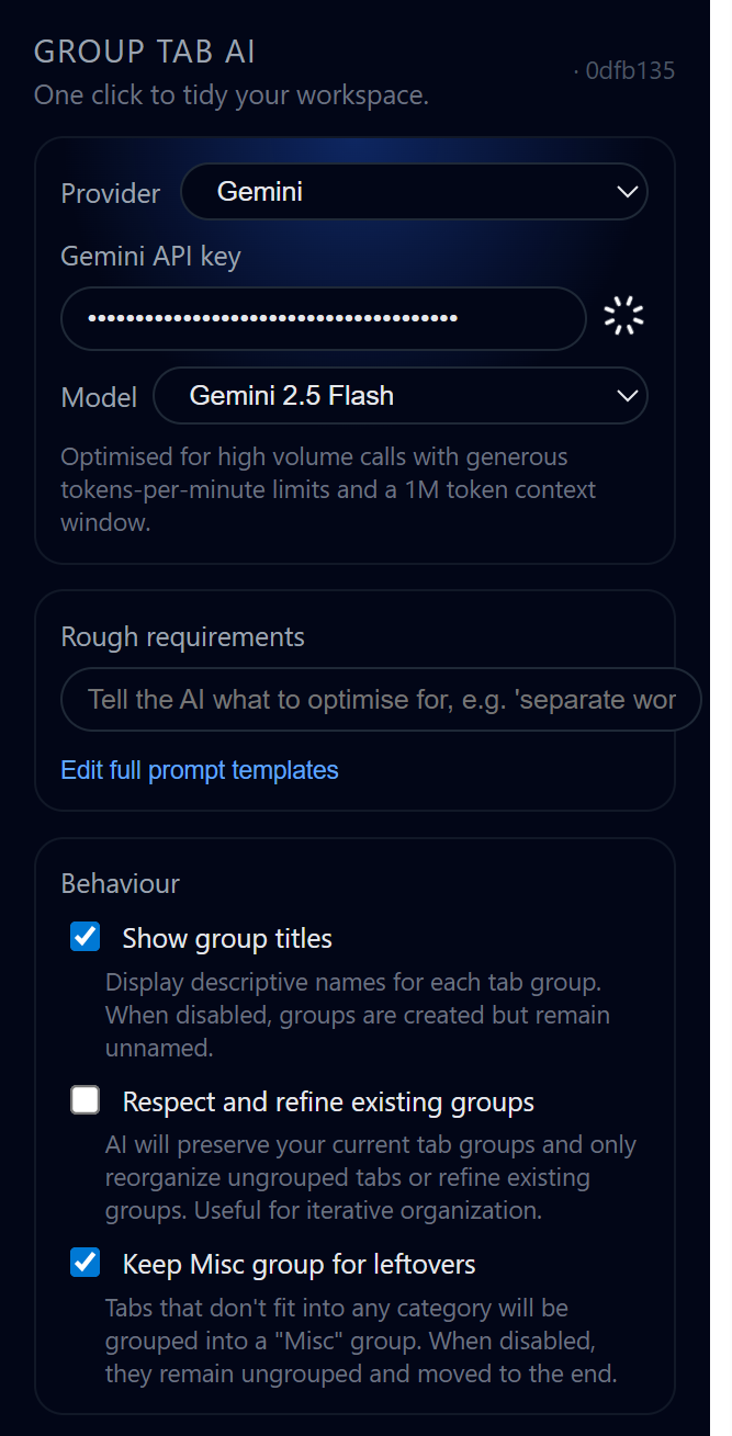
It sends that data to an LLM (I set it up to work with either OpenAI or Gemini). Because it reads the content, it can tell that a GitHub page for a “React Library” is different from a GitHub page for “Tracking Issues.”

I’m using Google Gemini 2.0 Flash for this mostly, with the thinkingBudget set to 0. It’s fast enough that by the time I blink, the tabs are sorted.

I spent nights tweaking prompts to make it focus on tasks, not domains with extra context from the website contents along with careful prompt to let them reasoning and choose. For example, if you’re a dev, it might make groups like “Bug Hunting” or “API Docs.” Designers get “Mockups” or “Inspo.” It works for anyone,

students with class notes, marketers with campaigns.

image 10 - quochung.cyou PTIT

The feature I actually wanted: It learns

This is the part I’m most proud of. I know AI isn’t perfect. It’s going to mess up. It might group a design blog under “Development” instead of “Inspiration.”

Usually, with AI tools, you just have to live with the bad output. But I built a Learning System into this.

  1. If the AI groups something wrong, I manually move the tab to the right group.
  2. The extension records that move.
  3. After I’ve corrected it a few times, I can click a button to “Analyze Behavior.”
  4. The system looks at my corrections and rewrites its own system prompt.

Next time I run it, it knows: “Oh, he likes to keep his ‘Localhost’ tabs separate from his ‘Production’ tabs,” because it updated its own instructions based on my manual fixes.

The Tech Stack

For the frontend devs out there, I built this using Plasmo. It’s basically the Next.js of browser extensions, makes working with React and TypeScript in a chrome-extension environment actually bearable.

Everything is local. Your API keys are stored in your browser, and the learning data (your grouping habits) stays on your machine.

Try it out

It’s open source (GPL-3.0). I built it because I needed it, but if you’re tired of domain-based grouping that doesn’t actually help, give it a shot.

https://github.com/quochung-cyou/group-tab-ai-extension

Releases: https://github.com/quochung-cyou/group-tab-ai-extension/releases/

FOSSASIA 2024 Hackathon: Housing Connector

image 1 - quochung.cyou PTIT

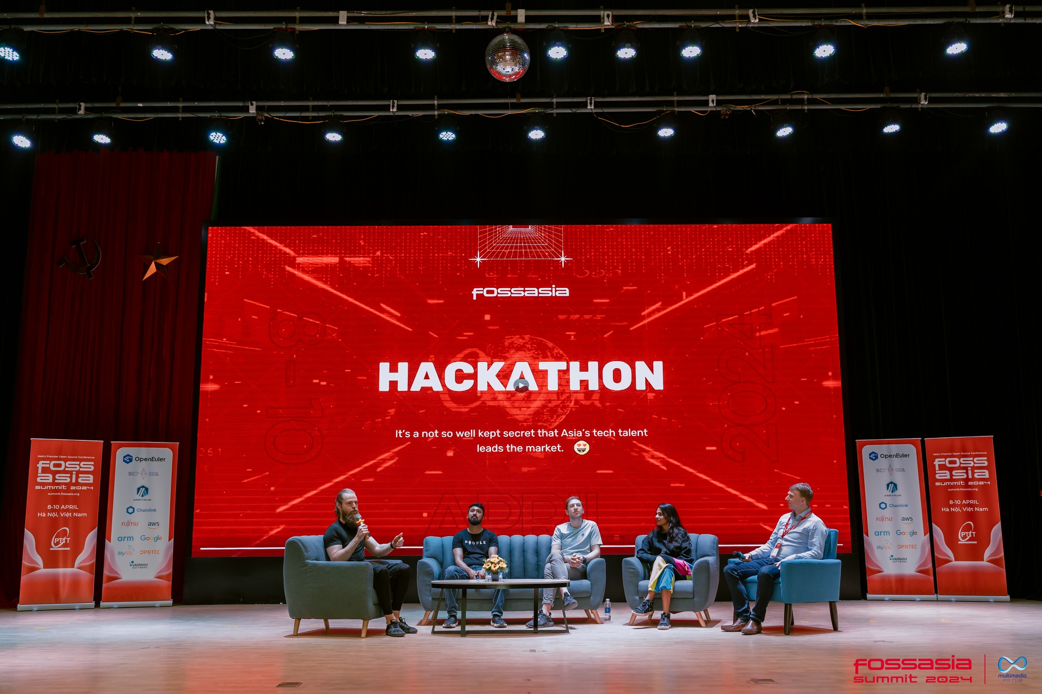
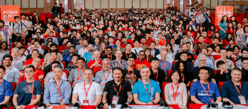
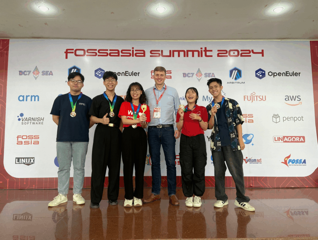
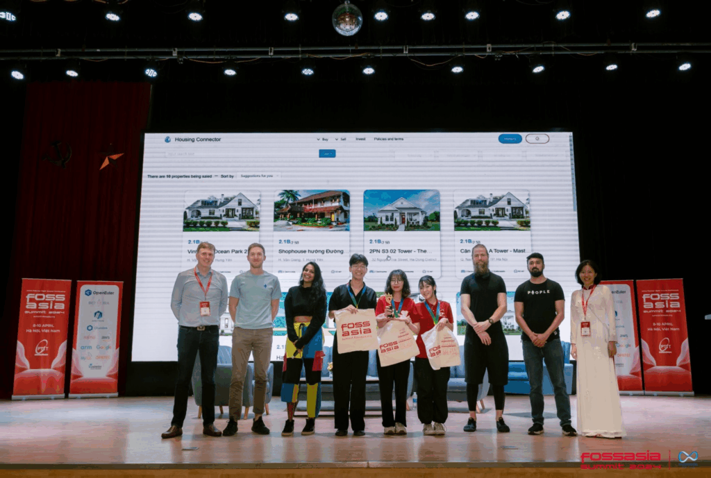
The atmosphere at the FOSSASIA Summit 2024 was absolutely electric. Hosted at PTIT, it’s a massive gathering with over 5,000 people from 50 countries, 200+ speakers from giants like Google, Huawei, and Oracle,…. Amid all that, there’s this Web3-focused hackathon, sponsored by Chainlink and Devfolio, challenging devs to build real-world blockchain solutions in just 48 hours.

image - quochung.cyou PTIT

The idea came from what I see at work. Vietnam’s real estate is growing fast, the market’s supposed to double in size soon, with more young people in their 20s and 30s wanting in. But buying property? It’s expensive, and if you team up with friends or family, contracts get messy with arguments and risks. A lot of folks are shopping online now like 70% or something but trust is low. So, we made Housing Connector: a platform where small investors can pool money for properties, connect with agents, and use blockchain to keep everything clear and safe.

image 5 - quochung.cyou PTIT
image 4 - quochung.cyou PTIT

Basically, it works like this: Investors check out listings with details on location, costs, potential returns. They chip in what they can, sign smart contracts through Chainlink so no one’s getting screwed. When the property sells, money gets split automatically, minus a small fee, that’s how the app makes money. Agents get leads and data to sell better, and as more join, it pulls in more investors and properties. It’s a loop that could grow quick. We used React for the front end, Solidity for contracts, and stuff like Ethereum and Web3.js. Nothing fancy, just enough for a basic demo.

image 6 - quochung.cyou PTIT
image 7 - quochung.cyou PTIT

We submitted right at the deadline: a POC where you could “buy” a apartment in Hanoi with pooled funds. Out of over 1,000 people and 43 teams, they picked us as winners!

image 3 - quochung.cyou PTIT
image 2 - quochung.cyou PTIT

Honestly, it taught me a lot about teamwork under pressure. We’re proud of the prototype, even if it’s rough – built in two days, after all. Maybe we’ll keep working on it, add more features like AI for price predictions. Shoutout to FOSSASIA for the event!!!

Chung kết ACM/ICPC PTIT 2023

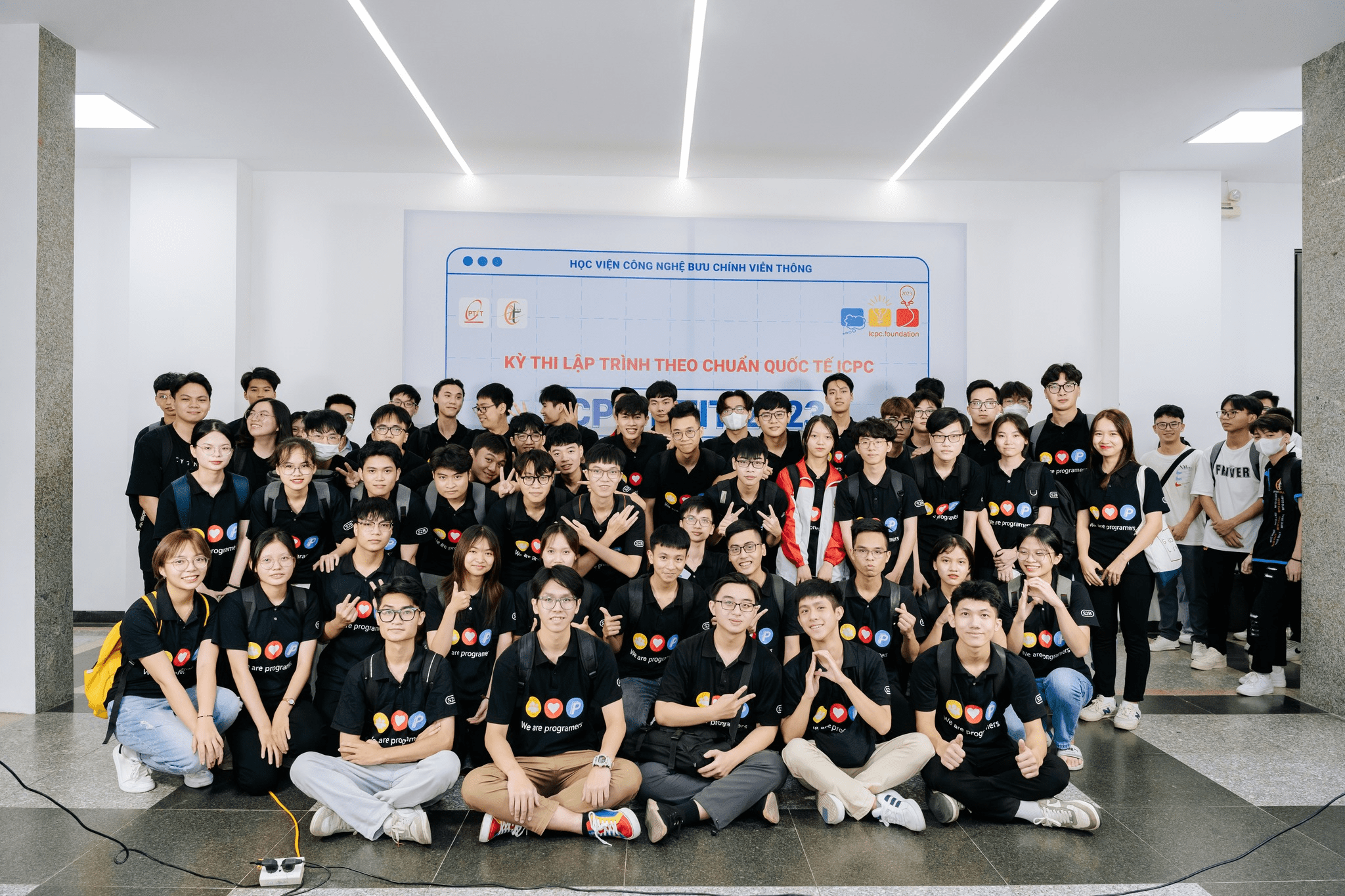
Vào ngày 24/09/2022, Học viện Công nghệ Bưu Chính Viễn Thông đã tổ chức kỳ thi chung kết ICPC PTIT 2022. Sự kiện này đã thu hút 41 đội xuất sắc từ hơn 180 đội tham gia (không tính miền Nam). Kỳ thi đã diễn ra tại sảnh A2 của Học viện. Trong kỳ thi năm 2023, có sự tham gia đáng kể của các sinh viên khoá D22 và E22 (năm nhất). Đây là năm thứ hai mình tham gia cuộc thi này, và từ kinh nghiệm năm ngoái, mình đã có một số kinh nghiệm nhất định :v

image 18 - quochung.cyou PTIT

Đội của chúng mình, có tên là “ProPTIT. Ba bà đi bán lợn con”, gồm ba thành viên: Nguyễn Quốc Hưng (E2105), Nguyễn Mai Phương (D21CN01) và Lê Trí Tâm (D21). Sau khi đứng top 20 trong gần cả cuộc thi, chúng mình đã lội ngược dòng vào 15 phút cuối để giải lên 5 bài và giành được top 4 chung cuộc.

Đề thi năm 2023 có nhiều thay đổi so với 2022, nhìn chung các bài năm nay có nhiều đổi mới, tập trung vào giải thuật nhiều hơn, độ khó cũng khó hơn hẳn năm ngoái. Chắc đây cũng là một phần lí do số sinh viên năm nhất vào chung kết khá ít, chỉ có khoảng 1-2 bài cơ bản và còn lại là các bài với các thuật toán kinh điển như Quy hoạch động, dijkstra, greedy.

Một vài hình ảnh đáng chú ý trong kì thi

Thầy Cường và thầy Sơn tại vòng loại kì thi
Đội hình CLB Lập Trình PTIT checkin vòng loại
image 21 - quochung.cyou PTIT
khu vực thi 2023 tại hội trường a2
image 23 - quochung.cyou PTIT
image 24 - quochung.cyou PTIT

Một số nguồn tài nguyên cho lập trình Game

I. itch.io

Itch.io là một nền tảng cung cấp cho các các lập trình viên game hàng ngàn tài nguyên chất lượng cao để tạo ra những tựa game độc đáo. Nền tảng này cho phép bạn tải xuống các tài liệu như texture nhân vật, item, phong cảnh, map (tile sets), các hiệu ứng kĩ năng (skill effect) và rất nhiều thứ khác nữa để giúp bạn xây dựng một thế giới game hoàn hảo của mình.

- quochung.cyou PTIT

II. Gamefresco.com 

Gamefresco, một nền tảng chia sẻ và tạo đồ họa game mới được tạo bởi các game artist, đã công bố ra mắt phiên bản beta vào ngày 1 tháng 2 năm 2023. Gamefresco cung cấp một cách mới để chia sẻ các bộ sưu tập tài sản game chất lượng cao, bao gồm icon, nhân vật, môi trường map và background, cùng nhiều thứ khác.

Với Gamefresco, các nhà phát triển game và thiết kế game có thể khám phá, thu thập và chia sẻ các tài nguyên game từ khắp nơi trên thế giới. Có thể tạo ra bộ sưu tập của riêng mình từ các tài nguyên của nhiều người khác nhau (Giống Pinterest).

745cbcaf666b48cc91941776b52126e5.Gamefresco The ultimate source for Free 2D game asset - quochung.cyou PTIT

III. GameDevMarket

GameDev Market là một marketplace tài nguyên lớn dành cho các nhà phát triển indie với nhiều tài nguyên game miễn phí và cả trả phí. Các nhà thiết kế đồ hoạ game khác nhau có thể đăng tải các gói tài nguyên theo chủ đề cùng với các tài nguyên game miễn phí mà bạn có thể tải về tham khảo. Tương tự như Itch.io, bạn có thể tìm thấy tất cả các loại tài sản game. Có các danh mục như 2D, 3D hoặc GUI, …. Có nhiều loại tài nguyên game khác nhau như background, nhân vật, xe cộ, quái, npc, môi trường, cây cối và nhiều hơn nữa.

Gamedevmarket free game art - quochung.cyou PTIT

IV. OpenGameArt

Open Game Art free game art 1024x569 1 - quochung.cyou PTIT
generic platformer mockup - quochung.cyou PTIT

Một trang có giao diện trông có vẻ hơi lỗi thời một chút, tuy nhiên tại đây có rất nhiều tài nguyên miễn phí để làm game. Đa số tài nguyên đều nằm trong bản quyền chung nên bạn có thể sử dụng trong các dự án mang tính thương mại mà không cần để lại credit. Ngoài ra cộng đồng trên đây cũng khá active và bạn có thể theo dõi và lọc theo đánh giá của cộng đồng. Thường thì các tài nguyên nổi tiếng và được đánh giá cao sẽ được hiện trước

V. CraftPix

Craftpix free game art 1024x488 1 - quochung.cyou PTIT

Cũng như đa số các trang bên trên. CraftPix là một marketplace chứa cả các tài nguyên miễn phí và trả phí. Tại đây bạn có thể tìm các asset 2D cho game arcade, chiến thuật, platform, rpg, … CraftPix có một đặc trưng là các asset đều mang một sắc màu độc đáo. Nếu bạn đang muốn tạo một con game mang tính sáng tạo và lạ thì có thể thử trang này

Cảm quan và review chung về Suzume no Tojimari – Khoá chặt cửa nào Suzume!

Cuối cùng thì thông tin chính thức về ngày phát hành của Suzume no Tojimari, tác phẩm mới nhất từ đạo diễn Makoto Shinkai đã được hé lộ khiến các fan háo hức mong chờ.

Khoá chặt cửa nào Suzume!

Doanh thu của Suzume chính thức vượt mặt bộ phim nổi tiếng của MAPPA để  đứng thứ 9 tại Nhật Bản | ONE Esports Vietnam

Nội dung movie tập trung vào Suzume, một cô gái 17 tuổi gặp một chàng trai trẻ đang tìm kiếm cánh cửa. Suzume tìm thấy một cánh cửa kỳ lạ giữa đống đổ nát và mở nó ra. Nhưng vì lý do đó nhiều cánh cửa bắt đầu mở ra trên khắp Nhật Bản, gây ra thảm họa. Bây giờ, Suzume phải đóng cửa tất cả chúng để cứu Nhật Bản.

Doanh thu của Suzume chính thức vượt mặt bộ phim nổi tiếng của MAPPA để  đứng thứ 9 tại Nhật Bản | ONE Esports Vietnam

Đây là tác phẩm mới nhất do “phù thủy của những nỗi buồn” Makoto Shinkai viết kịch bản và đạo diễn, và cũng là tác phẩm tiếp theo kể từ Weathering with You (2019). Phim có sự tham gia lồng tiếng của Nanoka Hara và Hokuto Matsumura, với thiết kế nhân vật của Masayoshi Tanaka, chỉ đạo hoạt hình của Kenichi Tsuchiya, chỉ đạo nghệ thuật của Takumi Tanji, và âm nhạc của Radwimps và Kazuma Jinnouchi.

Suzume no Tojimari tung teaser trailer với phần hình ảnh 'trên cả tuyệt vời'

Phim kể về Suzume, một cô gái 17 tuổi sống tại thị trấn yên tĩnh tại vùng Kyushu, phía Tây Nam Nhật Bản. Câu chuyện bắt đầu khi Suzume gặp được một chàng trai trẻ đang tìm kiếm một “cánh cửa”. Cả hai đã đi cùng nhau và tìm thấy được một cảnh cửa cũ tại một căn nhà bỏ hoang trên núi. Như thể bị thứ gì đó lôi kéo, Suzume đưa tay ra phía cánh cửa và cũng từ đây, những biến cố không may xuất hiện trên khắp Nhật Bản.Bộ phim là hành trình xuyên Nhật Bản để khóa những “cánh cửa tai ương” đồng thời cũng là cuộc phiêu lưu và chiến đấu ở thế giới hiện đại để tìm kiếm sự trưởng thành và sự tự do của một cô gái.Về dàn diễn viên lồng tiếng thì:Nanoka Hara trong vai Suzume IwatoHokuto Matsumura trong vai Sota MunakataEri Fukatsu trong vai Tamaki IwatoShota Sometani trong vai Minoru OkabeSairi Ito trong vai Rumi NinomiyaKotone Hanase trong vai Chika AmabeKana Hanazawa trong vai Tsubame IwatoMatsumoto Hakuo II trong vai Hitsujiro Munakata

Cốt truyện và tình tiết diễn ra khá nhanh và mạch lạc

Bộ phim khá dễ để nắm bắt cốt truyện, cho phép cả những người lần đầu xem phim có thể nắm được tình tiết dễ dàng. Tuy nhiên do câu truyện diễn ra khá nhanh và theo mình cảm thấy thì nó đi hơi nhanh nên người xem chưa thực sự cảm thấy chiều sâu của cảm xúc, các tình tiết tiếp theo khá dễ đoán và diễn ra theo motip chung của các sản phẩm khác của Makoto Shinkai gần đây.

Visual hình ảnh nhân vật
image - quochung.cyou PTIT

Là một đứa con được ra mắt vào năm 2023, bộ phim được trau chuốt khá kĩ về mặt hình ảnh và nhân vật. Các nhân vật đều có một màu sắc rất tươi đẹp, hình ảnh các cuộc sống đời thường, thành phố lớn tại Nhật Bản hay khung cảnh cao trào bộ phim đều có thể dễ dàng làm một bức ảnh nền nhờ hình ảnh của nó. Tuy vậy, nếu so sánh với Weathering with you của đồng tác giả, mình thấy hình ảnh của Weathering with you có phần nhỉnh hơn.

Suzume no Tojimari có after credit không?

Bộ phim sẽ không có After Credit ở cuối phim nên bạn có thể ra về và gửi tặng bộ phim một tràng pháo tay khi credit xuất hiện ;>

Cốt truyện tóm tắt chữ

Ở một thị trấn nhỏ ven biển ở Miyazaki, Suzume mơ thấy mẹ cô đưa cho cô một chiếc ghế gãy trong một thế giới kỳ ảo. Một buổi sáng, cô gặp một chàng trai trẻ đang tìm kiếm những nơi đã bị bỏ hoang. Cô nói với anh về một khu nghỉ dưỡng suối nước nóng (onsen) cũ. Nghĩ rằng mình đã gặp anh ấy trước đây, cô cũng đến đó. Tuy nhiên, thay vào đó, cô tìm thấy một cánh cửa. Sau khi mở cửa, cô tìm thấy thế giới giống với trong giấc mơ của mình, nhưng lại không thể bước vào đó. Khi thử lại, cô vấp phải một viên đá (keystone). Nhặt nó lên, nó biến thành một con mèo con và bỏ chạy. Trong sự bối rối và sợ hãi, cô bỏ chạy và quay lại trường.

Khi đang ăn trưa, Suzume nhìn thấy khói bốc lên từ khu nghỉ dưỡng trước khi một trận động đất nhỏ xảy ra. Cô chạy ra rồi nhìn lại, cột khói bây giờ đã là một cột màu đỏ kéo dài lên trời. Lo lắng, cô chạy đến khu nghỉ dưỡng thì thấy khói bốc ra từ cửa và chàng trai trẻ cô thấy trước đó đang cố gắng đóng cánh cửa lại. Thấy anh bất lực, Suzume chạy đến giúp anh, rồi khói rơi xuống gây ra một trận động đất lớn. Anh vẫn cố gắng đóng cửa lại, nhưng bất chấp sự phản đối của anh ấy, Suzume vẫn giúp anh đóng cửa. Sau đó, sau khi nghe những cuộc trò chuyện từ thuở hoàng kim của khu nghỉ dưỡng, họ cuối cùng đã đóng được cửa và chàng trai đó khóa cửa bằng chiếc chìa khóa trên cổ. Sau đó, cái cột màu đỏ biến mất và trời mưa trong một thời gian ngắn. Suzume đưa người chàng trai về nhà, và anh ta tự giới thiệu mình là Sōta Munakata. Anh ta nói với Suzume rằng anh ta phải tìm và khóa cửa ở những nơi bỏ hoang để ngăn “sâu” từ thế giới ma thuật gây ra động đất. Sau đó, một con mèo xuất hiện và biến Sōta thành chiếc ghế trẻ em mà anh đang ngồi. Quá tức giận, “chiếc ghế” đuổi theo con mèo, theo sau là Suzume. Cô đuổi theo họ đến một chiếc phà hướng đến Ehime, nhưng hắn trốn thoát lên một chiếc thuyền khác, khiến họ mắc kẹt. Đêm đó, Tamaki, dì của Suzume, yêu cầu cô ấy quay lại, nhưng cô lại cúp máy. Sau đó, Sōta nói với cô rằng con mèo đã từng là một viên đá, và những con sâu đã được giải phóng ngay cả khi nó được loại bỏ.

Họ đi đến Ehime. Sử dụng manh mối từ những người dân địa phương đã chụp ảnh và đặt tên cho con mèo là “Daijin”, họ lần theo con mèo. Suzume hỏi một cô gái, Chika, nếu cô ấy nhìn thấy Daijin, nhưng một trận động đất cắt ngang họ. Nhìn thấy một con sâu đang nổi lên, Suzume bỏ chạy, và Chika mời cô ấy đi nhờ trên chiếc xe tay ga của mình. Họ tìm thấy một ngôi trường bỏ hoang, và Suzume chạy vào. Sōta không tự đóng được cửa và chìa khóa của anh bị thổi bay. Suzume sau đó nhặt nó lên. Cần sự giúp đỡ của cô, Sōta bảo Suzume hãy tưởng tượng về thời hoàng kim của ngôi trường, rồi họ đã khóa cánh cửa thành công, xua đuổi con sâu. Sáng hôm sau, sau khi ở lại nhà trọ của gia đình Chika và trở thành bạn với cô, họ chia tay nhau.

image 6 - quochung.cyou PTIT

Trong một cơn bão khi đang đi đến dịa điểm tiếp theo, Suzume và Sōta trú tại một trạm xe buýt. Rồi một người phụ nữ tên Rumi dừng lại và cho họ đi nhờ. Trong khi đang dừng chân, Rumi chỉ ra công viên giải trí bỏ hoang gần thị trấn. Suzume tình nguyện trông cặp song sinh của cô ấy khi Rumi phải đi làm, Sōta cũng giúp cô. Khi cặp song sinh chìm vào giấc ngủ, Suzume lại giúp Rumi tại quán bar của cô ấy, lúc đó cô ấy để ý thấy Daijin. Trong khi cô và Sōta đuổi theo hắn, một con sâu mới xuất hiện, Sōta đành chia ra để đuổi theo con mèo. Suzume tìm thấy cánh cửa gắn với buồng của đu quay, nhưng Sōta vô tình kích hoạt nó, và Suzume bước vào sau khi nhìn thấy thế giới trong mơ. Trong khi đó, Sōta yêu cầu Daijin biến trở lại thành viên đá, nhưng hắn từ chối, muốn “chơi” Suzume. Suzume, sau khi được Sōta giúp đỡ, sau đó khóa cửa lại. Trên buồng, Suzume kể cho Sōta nghe về thế giới giấc mơ và mẹ của cô. Khi họ ngủ, Sōta đang mất dần ý thức về bản thân trong hình dạng chiếc ghế của mình, khi ở Miyazaki, Tamaki quyết định tự mình đưa Suzume trở lại sau khi nhận được lời khuyên từ Minoru, đồng nghiệp của Tamaki.

Ngày hôm sau, Suzume và Sōta đến căn hộ của Sōta ở Tokyo. Ở đó, anh kể cho cô nghe câu chuyện thần thoại về Namazu và viên đá trung tâm nằm ở Tokyo, rằng nó đã mất tích, và nếu con sâu của Tokyo xuất hiện, Nhật Bản sẽ bị hủy diệt. Gia đình anh đảm bảo rằng tất cả các cánh cửa vẫn được khóa, và anh đã vác gánh nặng đó từ người ông đang nằm viện của mình. Tuy nhiên, họ không biết cánh cửa của Tokyo ở đâu. Sau đó, bạn của Sōta, Tomoyo Serizawa, sau khi gõ cửa, nói với Suzume để cho Sōta biết rằng anh muốn nói chuyện với anh ấy, nhưng Suzume nhìn thấy một con sâu gần đó. Cô chạy ra ngoài, và Sōta đuổi theo Daijin sau khi gặp lại hắn, nhưng Daijin nói rằng Sōta phải trở thành viên đá mới để ngăn chặn con sâu. Sau khi tìm thấy con sâu, Sōta cảm ơn Suzume và trèo lên nó. Suzume đi theo anh ta, và họ đã lên đến đỉnh của con sâu. Ở trên đó, Sōta biến thành viên đá trong tay Suzume, và Suzume cầu xin anh quay lại khi con sâu bắt đầu rơi xuống. Vì trận động đất sẽ giết chết nhiều người, Suzume đã rơi nước mắt đặt viên đá xuống. Suzume sau đó tỉnh dậy trong một hang động, nơi cô tìm thấy cánh cửa của Tokyo. Trong giấc mơ, cô nhìn thấy viên đá Sōta và cố gắng cứu anh ta, nhưng bất thành. Bất chấp lời cầu xin của Suzume, Daijin nói rằng không thể cứu được Sōta. Không nản lòng, Suzume đành nhờ ông nội đang nằm viện của Sōta, Hitsujirō, giúp đỡ, nhưng ông ấy cũng nói như vậy. Tức giận, Suzume nói rằng cô ấy sẽ bước vào thế giới giấc mơ và cứu anh ta. Nhận ra rằng cô đã từng ở đó trước đây, Hitsujirō nói rằng để vào được, cô phải tìm thấy cánh cửa đầu tiên mà cô đã bước vào.

Suzume bắt đầu hành trình trở về quê hương của cô ở Tōhoku, nơi đã bị phá hủy trong trận sóng thần Tōhoku năm 2011. Serizawa nói với cô rằng cô có thể sử dụng chiếc xe của anh ấy để tìm Sōta, nhưng Tamaki xuất hiện và yêu cầu Suzume về nhà với cô ấy. Khi cô từ chối, Tamaki quyết định tham gia cùng cô, nhưng Suzume không nói lý do rời đi của cô. Daijin cũng âm thầm đồng hành cùng cả ba. Khi xe của Serizawa bị hỏng, họ tấp vào một trạm dừng nghỉ. Tamaki gợi ý đi xe buýt đến Tokyo mà cô biết được từ Minoru, nhưng Suzume từ chối, giận dữ nói rằng Tamaki không phải mẹ cô. Quẫn trí, Tamaki nói với Suzume rằng cô hối hận vì đã nuôi nấng cô ấy. Sau khi Daijin rít lên, Suzume nhận ra rằng Tamaki đang bị chiếm hữu bởi con mèo đen Sadaijin. Tamaki, lúc này rất hối hận, chạy về điểm dừng chân. Sáng hôm sau, họ tiếp tục lái xe, nhưng Serizawa đã gặp tai nạn sau khi nghe lũ mèo nói chuyện. Suzume sau đó chạy về phía trước và Tamaki đuổi kịp trên một chiếc xe đạp cũ. Cô ngồi sau Tamaki và nói cho cô ấy biết bản chất của lũ mèo. Rất vui vì cháu gái đã tin tưởng mình, hai người đã hòa giải. Khi họ đến nơi, cô tìm thấy trong một trang trong cuốn nhật ký cũ của mình về cánh cửa trong một viên nang thời gian (time capsule). Ở ngưỡng cửa, Suzume bước vào thành công sau khi nói với Tamaki rằng cô ấy sẽ cứu người mình yêu.

Thế giới tràn ngập những con sâu. Sōta, trong trạng thái bế tắc, hồi tưởng về Suzume. Tuy nhiên, khi nghe thấy giọng nói của cô, anh đưa tay ra và cô kéo anh lại. Không còn là viên đá nữa, anh ta trở lại nguyên hình của mình. Tuy nhiên, kết quả là Daijin trở lại thành viên đá. Để ngăn chặn những con sâu, Sōta cầu nguyện và mang quá khứ về quê hương của Suzume trở lại. Sadaijin sau cũng hóa đá. Với hai viên đá trong tay, Suzume và Sōta phong ấn những con sâu và mang lại hòa bình cho thế giới mộng tưởng. Sau đó, Sōta để ý đến một đứa trẻ, Suzume từ 12 năm trước, và Suzume nhớ lại lần đầu tiên cô bước vào giấc mơ. Cầm lấy chiếc ghế, cô chạy đến chỗ cô bé, người đã nhầm lẫn cô với mẹ cô ấy. Suzume nói với cô ấy rằng cô không phải mẹ của cô ấy, khiến cả hai Suzume đều suy sụp. Cô nhường ghế cho Suzume trẻ và nói với cô ấy về tương lai của mình. Suzume trẻ hỏi cô ấy là ai, và cô trả lời, “Suzume của ngày mai”. Suzume trẻ rời khỏi thế giới giấc mơ, theo sau là Suzume và cả Sōta. Sōta trở lại Tokyo, và Suzume trở lại Kyushu cùng Tamaki, trên đường đi thăm những người bạn mới của cô ấy. Sau đó, Suzume đang trên đường đến trường thì lại thấy Sōta đang đi trên con đường mà họ gặp nhau lần đầu.

Cảm hứng câu truyện

Shinkai Makoto cho biết tại buổi họp báo sản xuất cảm hứng sáng tác tác phẩm này của anh đến từ cảm giác suy giảm mà anh cảm thấy khi thực hiện chuyến đi đến nhiều vùng khác nhau của Nhật Bản vì công việc, và nhận thấy rằng dân số giảm và không gian xanh tăng lên, còn cảnh tượng ở Shinjuku vốn đông đúc người qua lại trở nên im ắng trong đợt dịch viêm phổi truyền nhiễm, điều này đã nhắc nhở anh khi mọi người khai hoang vùng đất, họ tôn thờ vị thần của vùng đất và họ rời đi mà không làm gì cả, từ việc suy nghĩ về nơi mà những tàn tích nhân tạo này biến mất đã truyền cảm hứng giúp anh tạo nên nhân vật Suzume đến những nơi khác nhau của Nhật Bản để kết bạn với những người khác. Shinkai Makoto nhận xét mặc dù cốt truyện và nhân vật hoàn toàn khác nhau, tuy nhiên bộ phim này vẫn bị ảnh hưởng sâu sắc bởi tác phẩm anime điện ảnh Dịch vụ giao hàng của phù thủy Kiki của Miyazaki Hayao. Anh giải thích lần này anh không chỉ muốn sản xuất một tác phẩm có thể là lý do để khán giả đến rạp, mà còn muốn tạo ra một cực độ cho phép mọi người đắm chìm vào câu chuyện bất kể hình ảnh và âm thanh, trong phần tái bút của phiên bản tiểu thuyết, anh nói thêm trong quá trình hình thành cốt truyện của phim, anh đã nhớ lại hậu quả của trận động đất và sóng thần Tōhoku năm 2011. Đây cũng là tác phẩm điện ảnh thứ ba mà Kawamura Genki hợp tác với Shinkai Makoto sau Your Name – Tên cậu là gì? và Đứa con của thời tiết.[25]

Vào ngày 25 tháng 10 năm 2022, Shinkai Makoto tiết lộ tại cuộc họp báo cáo hoàn thành bộ phim rằng khán giả chính của anh ấy chủ yếu là thanh thiếu niên và ngôn ngữ chung của trận động đất đang dần biến mất, vì vậy anh muốn nắm bắt thời gian để chia sẻ tâm tư cùng với khán giả. Anh giải thích vào tháng 3 năm 2021, anh đã nhìn thấy cảnh hoa anh đào nở rộ ở Tokyo trong đợt dịch viêm phổi truyền nhiễm, và nhận ra vẻ đẹp cũng như sự tàn nhẫn của thiên nhiên, vì vậy anh bắt đầu suy nghĩ về việc có thể sử dụng bộ phim dưới hình thức giải trí, làm cho sự bình tĩnh và sắc nét của nó thành một bộ phim.

Khá là tiếc nhưng có vẻ mình không thấy easter egg nào của các phim khác trong bộ phim lần này, không như Your Name đã được xuất hiện như 1 easter egg tại Weathering with you.